Since showing animations on the overhead in class is problematic, I have prepared this summary that you can use with the CD in the front jacket of your textbook. Animations can be quite useful in understanding the concepts behind fluid mechanics (1 picture = 1000 words), so I encourage you to take advantage of them as you read the text.
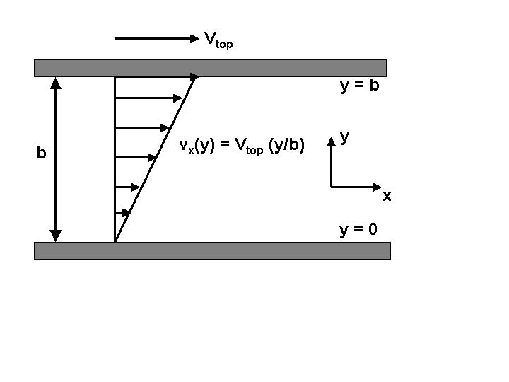
Question 3 deals with the simple flow system that we considered in class - the motion of fluid trapped between two plates, the bottom of which is stationary while the top moves at a known velocity in the x-direction. The geometry of this system is very simple, but it serves to introduce some common ideas in fluid mechanics - most importantly the property of viscosity.
In class we said that the fluid near the bottom plate will be stationary, because the collisions between the fluid molecules and the plate will oppose any net motion of the fluid. This is a typical property of fluid mechanics - when a fluid is near a solid wall, its velocity will match that of the wall (the "no-slip" condition).
So, if we want to predict how the fluid will move in the area between the two plates, we know first that at y = 0 (the bottom plate), the fluid will be at rest and at y = b (the top plate), the fluid will move at a velocity Vtop. The question is, what happens in the middle?
Viscosity, we have said, comes about from collisions between the molecules of the fluid in which some of the momentum of the fast moving molecules (found here at larger values of y) is transferred to the slower molecules at smaller values of y. This transfer of momentum from fast to slow regions has a "calming" influence on the flow, since it opposes any situation where a fast moving and slow moving region are in close contact. Because of viscosity, each "chunk" of fluid will tend to move at the same velocity as the surrounding "chunks".
How can we use this knowledge to predict how the average velocity of the fluid will change as a function of position for our flow example? Consider the following thin "slices" of fluid, each of thickness Dy, located around a distance y from the bottom plate. Because the molecules in the topmost slice are closer to the moving wall, we expect these molecules to be the fastest, with an average velocity vx(y+Dy). The molecules in the middle slice move somewhat slower, at a velocity vx(y), and the molecules in the bottom slice, being closest to the stationary wall, move at the slowest average velocity vx(y-Dy).
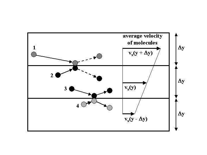
Because the molecules are moving around at random, we will have collisions between molecules in different slices. To see the effect of this, let's say that we have molecule 1, coming from the fast region so that it has a large velocity in the x-direction. When 1 collides with molecule 2, which being in the middle slice will be moving slower (on average), 1 will transfer some of its x-direction momentum to 2. Meanwhile, molecule 3 of the middle slice does the same thing to molecule 4 of the slow region. The net result is a continual transfer of momentum from the faster to the slower regions.
In the figure, I show that the velocity profile vx(y) is a linear function of y, which is equivalent to saying that vx(y) is equal to the average of vx(y+Dy) and vx(y-Dy). We can see why this should be the case by considering the collisions above. Let's say we try to increase vx(y) but keep the values of vx(y+Dy) and vx(y-Dy) the same. With this faster, larger value of vx(y), the difference in velocity between molecules 1 and 2 will be less, so there will be less momentum transferred into the middle slice from above. At the same time, the difference in velocities between molecules 3 and 4 will be greater when we "speed-up" the middle slice, so that more of the middle slice's momentum will be lost to the slice below. This means that because of this transfer of momentum (the property of viscosity), if the middle slice tries to speed up to a velocity larger than the average of those of the surrounding fluid, it will lose momentum and slow down. Of course, similar reasoning applies if we were to slow down the middle layer; then the effect of viscosity would be to speed it back up. This "averaging" process is what we mean by saying that viscosity has a calming influence on the flow, because it tends to make the flow of the fluid steady and smooth.
How can we apply this reasoning to predict the macroscopic velocity profile for the velocity of the fluid as a function of position? When we say vx(y), "the velocity of the fluid in the x-direction at a distance y from the bottom plate", what we mean is the average velocity of the many fluid molecules located in a "slice" (as in the diagram above) located at a distance y from the bottom wall. In liquids and gases (at least at near-atmospheric pressure), the fluid molecules only travel from between 1 Angstrom (10-10 meter) to 0.1 micron (10-7 meter) between collisions; distances far smaller that those that characterize the flow situations that we will consider in this class. For example, if we want to consider the flow of fluid between two parallel plates separated by a distance of 1 cm, this macroscopic (i.e. visible to the naked eye) distance is far larger (100,000 to 100,000,000 times larger) than the microscopic (i.e. you need a very powerful microscope to see) distance that the molecules travel (on average) between collisions.
Rather than try to predict the motion of every molecule in the fluid (an impossible task), we are content instead to describe only how the average velocity of the molecules changes as a function of position and time. While in our first two lectures, we have described fluids as being composed of molecules for the purpose of explaining the origins of pressure and viscosity, we will not discuss the molecular nature of fluids during the remainder of 10.301. Instead, we will derive the mathematical laws that describe how this average velocity of the fluid molecules changes as a function of position and time in various flow situations, using the familiar physical concepts of inertia, momentum, force, and acceleration. This method of "smearing-out" the motion of the individual molecules to model instead only their average velocity relies upon the vastly different length scales of the macroscopic flow geometry and the microscopic motion of individual molecules, and is known as continuum mechanics.
Now, back to the question of predicting the velocity profile vx(y) in our flow example. Because of viscosity, the transfer of momentum by collisions between molecules in the fluid, each "slice" will tend to have a velocity equal to the average of the velocities of the neighboring slices above and below. This characteristic is equivalent to saying that, in this example, the average fluid velocity is a linear function of position, and it yields the following mathematical form - the only linear function that satisfies the "no-slip" boundary conditions that the velocity is stagnant (non-moving) at the bottom plate (y = 0) and matches the velocity of the upper plate at y = b.
![]()
From this form of the velocity profile, observe that the greater the ratio Vtop/b, the greater will be the velocity difference between neighboring slices of fluid throughout the system. This is because in the collision diagram above, we have
![]()
If we then double the velocity gradient dvx/dy, we expect that for most fluids that there will be twice as much momentum transferred by the collisions, and so we will have to apply twice as large a force to the upper plate to keep it traveling at a constant velocity.
If we keep the distance b between the plates constant and double the velocity of the upper plate, we double the velocity gradient, since dvx/dy = Vtop/b, and so our reasoning says that the force on the upper plate would be twice as great. Likewise, we would double the force if we keep the upper plate velocity constant and decrease the distance b between the plates by a factor of two. We see therefore that from our simple (although probably not self-evident) reasoning, we expect for most fluids the following mathematical law for the force per unit area that must be applied to the top plate to keep it moving at a constant velocity.
![]()
To obtain this law, we have not assumed much about the detailed structure of the fluid - whether it is a fluid or gas, the density, etc. The only thing that we have assumed is that the rate of momentum transfer from the fast to the slow regions caused by collisions within the fluid will be proportional to the velocity difference between neighboring slices, and thus proportional to dvx/dy = Vtop/b. Because this is a very general assumption, that works well for many fluids of simple molecules (air, water, hydrocarbons), we can use mathematical law for many systems. The coefficient of proportionality, m, that appears in this law is a measure of the "strength" or "effectiveness" of momentum transfer within the fluid, and is the property that we define as the viscosity of the fluid. By taking a look at the dimensions of this expression, we can see that viscosity has the SI units Pa*s, where 1 Pa = 1 N/m2 is the unit of pressure.
As part of this discussion, we have said that if a "chunk" of fluid starts to move faster than its surroundings, then the effect of viscosity is to slow it back down. Of course, the effectiveness of this "calming" action depends on the magnitude of the viscosity. For example, let's consider again our three-slice example from the figure above. Let's say that we increase the velocity of the middle slice by a magnitude Dv, but keep the velocities of the upper and lower slices the same. Because of viscosity, it will tend to lose to the surrounding fluid the extra momentum that it has picked up at its new velocity, r(ADy)Dv. Here A is the area of our slices in the horizontal (x,z) plane. As we have said, the rate at which this momentum is lost through collisions with the surrounding fluid will be proportional to the viscosity, and to the local "gradient" (Dvx/Dy) in the velocity. If the rate of momentum transfer by viscosity is large compared to the total amount of momentum that must be transferred, the middle slice will quickly slow back down to its original velocity. If this is the case, we expect to see a velocity profile, vx(y), that is a nice, smooth function of position that does not change with time. Any departure from this steady velocity profile will be resisted very quickly by momentum transfer within the fluid from viscosity. Since in this situation, layers (in Latin lamellae) of the fluid tend to slide smoothly over each other, we call this situation laminar flow.
On the other hand, if the viscosity of the fluid is very low, then it is much easier to locally "speed up" the middle slice, because it takes a much longer time for the extra momentum to be transferred away to the surrounding slices. In this case, the "calming" effect of viscosity on the flow is much weaker, and we should not be surprised if our flow should have some local regions that move faster than other regions nearby. When this occurs, we observe irregular, complex flow patterns that change as a function of time, a condition known as turbulent flow.
It would be nice if, for a given flow geometry, we could calculate a single number that would tell us whether to expect the flow to be smooth (laminar) or irregular (turbulent). We want the value of this number to be independent of the system of units that we use, so that for a given situation, we would calculate the same numerical value regardless of whether we use english, cgs, or metric (SI) units. A small value of this number (say less than one) would indicate that the internal viscous forces in the fluid are very effective in keeping the flow smooth (laminar) and a large value (much greater than one) would signify that the "strength" of inertia is greater than that of viscosity, and that the flow may become turbulent.
Such a number is commonly calculated, and is named the Reynolds' number, Re, after the fluid mechanics researcher Osborne Reynolds.
![]()
Here, Dv is a characteristic difference in velocity between two regions of the fluid separated by a distance Dy. The greater the value of rDv, the larger is the difference in momentum of the different regions that must be transferred by viscosity to keep the flow "smooth". Of course, if we increase the viscosity, we increase the rate of momentum transfer and the flow will be smoother. Likewise, if we keep the density, viscosity, and Dv the same, but decrease Dy, the difference in velocities between nearby molecules will be greater and momentum transfer from collisions will be more rapid. This will tend to make the flow smoother, and promote laminar flow.
From these arguments, we see that when Re is small (Re << 1), we can be confident that the flow will be smooth (laminar) but when Re is large (Re >> 1), we may expect flow situations in which nearby "chunks" of fluid may move at very different velocities. This complex, erratic, flow behavior is known as turbulence. Typically, the transition from laminar to turbulent flow occurs over a range of Reynolds' numbers from 100 to 10,000. In the videos that we will view below, we will see clearly the distinction between laminar and turbulent flow, and why the Reynolds' number is so important to the study of fluid mechanics.
If we apply the concept of a Reynolds' number to the system of two plates shown above, we see that since the top plate is moving at a velocity Vtop and the bottom plate is stationary, then Dv = Vtop. Since the fast and slow regions are separated by a distance b, the spacing between the plates, we choose Dy = b. Then, for the case of flow between parallel plates, the Reynolds' number is
![]()
We will examine next the importance of the balance between inertia and viscosity, as represented by the Reynolds' number, by viewing videos of flow situations found on the CD in the front jacket of the text.
In this film, we see a solid sphere (a ball) floating in a bowl of liquid. This bowl sits on a turntable that can rotated at a constant number of revolutions per minute. Initially, the turntable is at rest, but then it starts to rotate.
For the first animation, we consider a fluid with a large viscosity such that Re = 0.3 < 1. Immediately after the turntable (and with it the bowl) begins to rotate, the fluid next to the bowl, because of the "no-slip" condition, will rotate at the same velocity. Since the fluid at the center of the bowl is still stationary, the effect of viscosity will be to transfer momentum from the edge to the center. When Re < 1, this transfer of momentum by viscosity occurs very rapidly, and we see that the ball appears to move at its final, constant value very quickly after the bowl starts to rotate. Likewise, when the bowl rotation is stopped, the ball also stops quickly. This immediate start and stop behavior is a consequence of the relative insignificance of inertia compared to the viscous forces in the system.
In the second animation, we perform the same experiment, but now with a fluid that has a lower viscosity (Re = 30 > 1). Now, the rate of the momentum transfer is weak compared to the effect of inertia, and the ball continues to move for a long time after the bowl has stopped rotating.
How do we calculate the Reynolds' number in this case? First, the density and viscosity are those of the fluid, of course. The difference in velocities between the stationary center and the moving edge of the bowl will be wR, where w is the angular frequency of the rotation and R is the radius of the bowl. Dy will be the bowl radius R, so the Reynolds' number will be
![]()
Here we observe the flow of a liquid through a pipe of diameter D caused by pushing the fluid through the pipe using a pump. Initially in this video, the pump only pushes the fluid through the pipe slowly, so that the inertia of the fluid is quite small. Near the wall of the pipe, the fluid is, by the "no-slip" condition, stationary, and it moves fastest along the centerline at a velocity v. The Reynolds' number is therefore defined as
![]()
When the fluid flows slowly through the pipe, the Reynolds' number is small and the viscous forces are strong enough, compared to the low amount of inertia, to keep the flow smooth (laminar). Dye introduced into the pipe upstream flows smoothly down the pipe, and is observed as a horizontal line.
As the video continues, the velocity of the fluid in the pipe is continually increased, until the Reynolds' number becomes much greater than 1. When this happens, the flow undergoes a transition (at Re ~ 1000) from a smooth, steady flow, to a complex flow pattern where the velocity appears to be an erratic function of position and time. This erratic flow, cause by strong inertia and weak viscosity, is called turbulence.
Obviously, the balance between inertia and viscosity is an important property in studying the motion of fluids, and will receive much attention in this course.
In the first video (4.5), we observe the motion of fluid around a collection of cylinders at moderate values of the Reynolds' number, where the flow is still quite smooth. This contrasts greatly with the second example (6.7), which shows the complex flow pattern found in turbulent flow around a cylinder at large Reynolds' numbers. On the "downstream" side of the cylinder, vortices are formed in a pattern that changes very irregularly as a function of time. Not surprisingly, the net force on the cylinder also fluctuates with time. The same phenomenon happens when moving air (the wind) flows around a traffic sign during a storm, in which case the time-varying force on the sign causes it to oscillate irregularly back and forth.