To start, let's consider why you would interpolate data. The most likely answer is that you could never sample adequately for all locations that you are interested in. Think of rainfall measurements. The older and more precise method of measurement involves rainfall gauges that need to be inspected at various points during a rainfall event. Because of data collection issues, such as the time to travel to each gauge and check the rainfall amounts, a limited number of rain gauges are used. Because there is a spatial correlation between rainfall amounts in various locations, it is assumed that rainfall gauges near each other have similar rainfall and that the rainfall amounts between rain gauges is similar to the rainfall amounts at the gauges. The further you are from a gauge, the less certain you are about the amount of rainfall at that location.
Predicting rainfall, elevation, or anything else, between locations where you have measurements, is spatial interpolation. It is possible to do this in ArcMAP and other GIS software. It is also possible to interpolate data in Matlab and in several statistical packes.
Interpolation is a large topic and this exercise is intended to introduce you to the concept within the context of a GIS.
Interpolating in ArcMAP
In this exercise, you will interpolate data using two of the three interpolation procedures available in ArcMAP, Inverse Distance and Kriging ( the third method is Spline interpolation ). You should look at the help system to see how these work. Additionally, there is much information in the literature on spatial interpolation. The choices you have in the software you are using are commonly found in most commercial GIS packages.
Preparing the data
Your data is rainfall data for a watershed in Jefferson County, Texas. It is annual precipitation to date for 2003. It is stored as T:\Lab11data\rainfall.dbf (you first need to attach th T: drive using the attach command in a Command Prompt window - attach -DT 1.963), and is a database file that you will need to add to you map and then convert to a point shapefile. There are four fields (columns) in the dbf:
You can see these fields in ArcCatalog, by finding the file, selecting it's properties, and looking at the Fields tab. You could also open the dbf in Excel or in Access to see the fields and the data. To load the data into ArcMap, you will have to figure out how to create points from the Latitude/Longitude coordinate data
Search the ArcMAP help for:
x,y coordinate data, adding to maps
and follow the directions. This process will create a temporary shapefile. The coordinates are latitude and longitude (LAT and LON) which should be the Y and X used in making this a shapefile, respectively. Edit the projection. Assume a geographic coordinate system using WGS-84 coordinates (found under Geographic Pojections >> World folder. Once you have created the point file, you should export it to a permanent shapefile before projecting.
Convert the shapefile you created to UTM Zone 15 North using ArcToolbox. Find the UTM projection in Defined Projections >> WGS 1984 >> WGS 1984 UTM Zone 15N. You will use this in the interpolation exercise.
Before you start, print out a map of the projected rainfall guages with the rainfall amount labeled. Try to quickly contour this data by hand, using a 2 inch interval. You will check this against the machine contour from interpolated data later in this exercise.
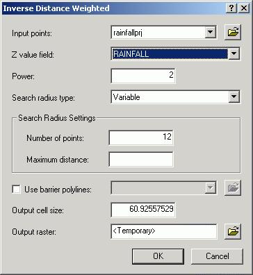
Inverse Distance Weighted Interpolation (IDW)
According to the ArcGIS help:
" IDW interpolation explicitly implements the assumption that things that are close to one another are more alike than those that are farther apart. To predict a value for any unmeasured location, IDW will use the measured values surrounding the prediction location. Those measured values closest to the prediction location will have more influence on the predicted value than those farther away. Thus, IDW assumes that each measured point has a local influence that diminishes with distance. It weights the points closer to the prediction location greater than those farther away, hence the name inverse distance weighted."
IDW is an inexact interpolation process. That is, the values that are interpolated won't exactly match the input points that are used.
To find the IDW method, go to Spatial Analyst >> Interpolate to Raster >> Inverse Distance Weighting. You can alter the power and the search radius settings - but be careful with the settings since this is a sparse dataset. Keep the default output cell size. Make sure you change the Z value field to RAINFALL.
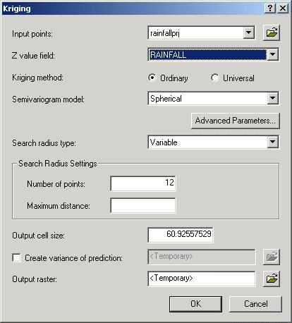
Kriging
From the Help pages:
"Like IDW interpolation, Kriging forms weights from surrounding measured values to predict values at unmeasured locations. As with IDW interpolation, the closest measured values usually have the most influence. However, the kriging weights for the surrounding measured points are more sophisticated than those of IDW. IDW uses a simple algorithm based on distance, but kriging weights come from a semivariogram that was developed by looking at the spatial structure of the data. To create a continuous surface or map of the phenomenon, predictions are made for locations in the study area based on the semivariogram and the spatial arrangement of measured values that are nearby."
Kriging is a complicated process and many papers have been written on how to use it to accurately interpolate a surface from a set of points. Nevertheless, it is commonly used and in its most simple for, Spherical Kriging, it can be used to interpolate without knowing all of the processes associated with it. Finally, Kriging can automatically produce a variance grid of how accurate the predictions are. This is useful to see how accurate the interpolation is away from the sample points. Kriging is an exact interpolator and returns the exact value for cells at the sample points.
To find the Kriging method, go to Spatial Analyst >> Interpolate to Raster >> Kriging. Make sure you change the Z value field to RAINFALL.
Machine contouring
Now check the contouring you did earlier in the exercise. Use the same process you used to create contours for DEMs. Create 2 inch rainfall contours for both your IDW and your Krieged surfaces. Print out your maps and compare the contours you drew against the machine contours.
Validation of Results
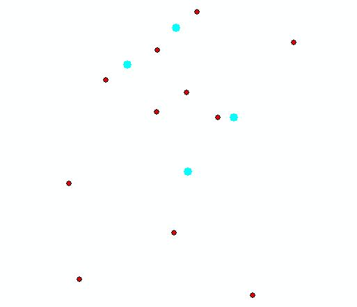
You will need to validate your results. In this case we have a small number of observations (15). Take out 4 of these and rerun your interpolations for both IDW and Kriging. Use the picture below to see which four points to remove from your projected shapefile. Keep all of the red points and remove (using the Editor toolbar) all of the blue points. Create a new shapefile with the four points missing.
An easier way to do this, without using the editor, would be to select the points you want to keep, and export the selected features to a new shapefile.
Once you have a shapefile with the four points removed, rerun the interpolations
for both IDW and Kriging, check the observed and predicted (or interpolated)
values at each of the removed points using the Identify tool. Use the original
projected shapefile to find the observed values.
Find the Root Mean Square Error (RMSE)
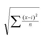
for the IDW and Kriging Interpolations, where (x - i) is the error at each of the four (n = 4) removed points. Which one is more accurate?
Created by Daniel Sheehan, 2003
Updated 10/29/03 -CA, 10/11/2006 -DS