Building Matrices

 

Everything in MATLAB is a matrix. A vector is a 1xN or Nx1 matrix; a scalar is a 1x1 matrix. The most straightforward way to make a vector or matrix is to write it out:

.1ex>> v = [1 2 3 4 5] creates the obvious vector (the spaces may be replaced with commas); the statements

.1ex>> m = [1 2 3; 4 5 6; 7 8 9] and

 .1ex>> m = [B<>1 2 3

		 4 5 6

		 7 8 9]

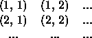
both create the obvious matrix. Note that semicolons are used to separate the rows of the matrix in the one-line square bracket notation.

It can be convenient to enter a complex-valued matrix or vector in the form

.1ex>> m = [1 2; 3 4] + i [4 3; 2 1] instead of the equivalent

.1ex>> m = [1+4i 2+3i; 3+2i 4+i] There are a number of useful functions to create a matrix from scratch. Specifically, zeros(M, N) and ones(M, N) create all-zero and all-one matrices respectively, eye(N) the size-N identity matrix, rand(M, N) a uniformly random matrix, randn(M, N) a normally distributed one, and hilb(N) a Hilbert matrix, among others. Some more specialized matrix generators are listed by help specfun. Those that take arguments (M, N) will create a square matrix if given only (N).

The function size takes a matrix and returns the vector [width height]; this can be used with other functions to build matrices the same size as existing ones, e.g.

.1ex>> emptym = zeros(size(m)) The length function gives the maximum of width and height.

Matrices and vectors may be built out of smaller ones;

.1ex>> va = [1 2 3]; vb = [4 5 6]; vc = [7 8 9];
.1ex>> m = [va; vb; vc]

produces the same matrix as before. Similarly, matrices can be built in blocks:

.1ex>> ma = [1 2; 3 4]
ma =


.1ex>> mb = [5 6; 7 8];
.1ex>> mwide = [ma mb]
mwide =


.1ex>> mtall = [ma ; mb]
mtall =

Since the size of a matrix can be changed at any time (and can be zero), things like this are valid:

.1ex>> x = [ ];
.1ex>> x = [x 1]
x =

.1ex>> x = [x 2]
x =

.1ex>> x = [x 3 x]
x =

Note that resizing a matrix does take time; doing it ten thousand times in a loop can be noticeable. A way to avoid this is to start with a matrix of zeros (or ones, as appropriate) of the eventual largest size, and then to use only part of the matrix at a time.

There are operations specifically to let you get a new object from an existing one; triu and tril take a matrix and produce its upper and lower triangular matrices. Diag takes a matrix and produces the vector of its diagonal entries, or takes a vector and produces a diagonal matrix with those entries. fliplr and flipud take a matrix and flip it left-right or up-down; rot90 takes a matrix and rotates it counterclockwise 90 degrees (an optional integer second argument specifies repetition). The operator ' takes the conjugate transpose of a matrix; the operator .' takes the transpose. The reshape function rearranges matrix elements into a new shape.

.1ex>> [1 2+i]'
ans =

-i

Elements of a matrix are referenced as m(row, column) (or v(n) for a vector); this can be used to access elements, or to build a matrix. Indexing starts at one, not at zero, so it looks like

You could, painfully, build a matrix like

.1ex>> m(1, 1) = 1; m(1, 2) = 2; m(2, 1) = 3; m(2, 2) = 4
m =

but this is more useful used in conjuction with for and while statements (see  Flow). On the other hand, submatrices can often be done this way quickly:

.1ex>> m = [1 2 3; 4 5 6; 7 8 9]; s = m([1 2], [2 3])
s =

The colon operator is critical to efficient use of MATLAB. The expression a:b evaluates to a row vector with values starting at a and incrementing by one as long as they are no greater than b. The expression a:s:b uses increments of s instead of one. A colon by itself as a matrix index, e.g. m(1, :) or m(:, 5), yields the entire row or column, while a colon used as the only index to a matrix turns it into a vector by stringing the columns together.

Also see help colon.

.1ex>> v = 1:5
v =

.1ex>> w = 5:-1:1
w =

.1ex>> m = [1 2 3; 4 5 6; 7 8 9];
.1ex>> s = m(1:2, 2:3)
s =


.1ex>> t = m(1:2, 3:-1:2)
t =


.1ex>> m(1:2, :)
ans =


.1ex>> m(:)'
ans =
In a similar fashion, linspace(low, high, n) gives a linearly evenly spaced vector of n points from low to high; n is 100 if omitted. Further, logspace(low, high, n) gives a logarithmically evenly spaced points between and (n defaults to 50); however, if high is pi, the high end is itself and not .

Finally, matrices can be loaded from a disk file created via MATLAB or some other application (e.g. a text editor); this is the fastest method for large matrices. If a file named base.extension contains a series of rows of numbers (no other formatting) defining a matrix, load base.extension will assign that matrix to the variable base. E.g. load values.txt takes data from the file values.txt and puts it into values. Don't use a .mat extension, since that will make load assume it is a MATLAB-saved file. Since load is frequently used for very large matrices, it does not echo the input.